Derivatives 🤔

Author

The majority of the text and code has been generated by AI.
Editor: Witek ten Hove

In mathematics, the derivative is a fundamental concept in calculus, describing the rate of change of a function at a particular point. Essentially, it gives you the “slope” of the function at that point. The concepts of partial derivatives and chain rule further extend this foundational concept.

Basic Understanding

The derivative of a function \(f(x)\) is given by the limit:

\(f'(x) = \mathop {\lim }\limits_{h \to 0} \frac{f(x + h) - f(x)}{h}\)

In Python, we can approximate this as follows:

Code

def derivative(f, x, h=0.00001):
    return (f(x + h) - f(x)) / h

This function can be used to find the derivative of a function at a given point. For example, if you have a function \(f(x) = x^2\), you can find the derivative at \(x=2\) like so:

Code

def f(x):
    return x**2

print(derivative(f, 2))  # Output: 4.00001

4.000010000027032

The derivative of \(x^2\) is \(2x\), so at \(x=2\), the derivative is \(4\). The output \(4.00001\) is slightly higher due to the approximation.

Partial Derivatives

A partial derivative is like a normal derivative but it’s used for functions with more than one variable. We consider one variable at a time and treat all other variables as constants.

For example, consider the function \(f(x, y) = x^2 + y^2\). The partial derivative of \(f\) with respect to \(x\) (denoted as \(\frac{\partial f}{\partial x}\)) is \(2x\), and the partial derivative with respect to \(y\) (denoted as \(\frac{\partial f}{\partial y}\)) is \(2y\).

In Python, you can approximate these as follows:

Code

def partial_derivative(f, x, y, h=0.00001):
    df_dx = (f(x + h, y) - f(x, y)) / h
    df_dy = (f(x, y + h) - f(x, y)) / h
    return df_dx, df_dy

def f(x, y):
    return x**2 + y**2

print(partial_derivative(f, 2, 3))  # Output: (4.00001, 6.00001)

(4.000010000027032, 6.000009999951316)

Chain Rule

The chain rule is a principle in calculus used to compute the derivative of a composition of functions. If you have a function composed of several other functions, the derivative of the overall function is the product of the derivatives of the component functions.

For example, if \(y = f(g(h(x)))\), then \(dy/dx = f'(g(h(x))) * g'(h(x)) * h'(x)\).

Consider the function \(f(x) = (3x + 1)^2\). Here, \(f(x)\) is a composition of \(u(x) = 3x + 1\) and \(v(u) = u^2\).

Using the chain rule to find the derivative:

Code

def f(x):
    return (3*x + 1)**2

def df(x):
    return 2 * (3*x + 1) * 3

print(df(2))  # Output: 42

We found \(df/dx = 2*(3x+1)*3\) by applying the chain rule: derivative of \(v(u) = u^2\) is \(2*u\), and derivative of \(u(x) = 3x + 1\) is \(3\). Thus, the derivative of \(f(x) = (3x + 1)^2\) is \(2*(3x+1)*3\).

So, the derivative of the function at \(x=2\) is \(42\).

Real World Applications

1. Business Management

In business management, derivatives can be used to optimize profit. Assume we have a function representing the profit of a company as a function of the price, \(f(p)\). The derivative \(f'(p)\) gives the rate of change of profit with respect to the price. If \(f'(p) > 0\), producing more units will increase profit, if \(f'(p) < 0\), producing more will decrease profit, and if \(f'(p) = 0\), we’ve reached a maximum or minimum point.

Take for instance the function \(f(p) = -p^2 + 20p\).

Code

import numpy as np
import matplotlib.pyplot as plt

def profit(p):
    return -p**2 + 20*p

prices = np.linspace(0, 20, 400)
profits = profit(prices)

plt.plot(prices, profits)
plt.title('Profit vs. Price')
plt.xlabel('Price')
plt.ylabel('Profit')
plt.grid(True)
plt.show()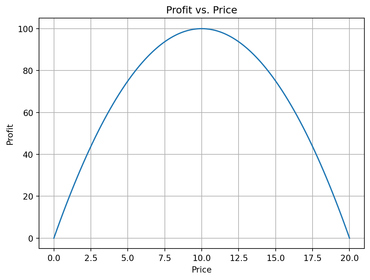

To find the price level that maximizes profits, we first obtain the derivative function \(f'(p) = -2p + 20\), solve the equation \(-2p + 20 = 0\) and check that the optimal price level \(p = 10\) results in a profit of \(-(10^2) + 20 * 10 = 100\).

Code

print(derivative(profit, 10))  # Output: almost zero

-9.99875737761613e-06

2. Engineering

In engineering, derivatives are used in areas like dynamics, control systems, and signal processing. For instance, in mechanical engineering, the velocity of an object is the derivative of the object’s position with respect to time.

3. Data Science

In data science, derivatives play a critical role in optimization algorithms, such as Gradient Descent used in Machine Learning. The derivative is used to determine the direction to move in the parameter space to minimize a given cost function.

For example, consider a simple linear regression model with one variable. The cost function \(J(m, b)\) for a given slope \(m\) and intercept \(b\) can be defined as the mean squared error (MSE) between the predicted and actual values. We can use gradient descent to find the \(m\) and \(b\) that minimize \(J(m, b)\), where the derivatives \(∂J/∂m\) and \(∂J/∂b\) guide the updating process.

Assignment

Basic: Make a short video explaining illustrating the functioning of the chain rule. Start by demonstrating that \((a + b)^2 = a^2 + 2ab + b^2\). For example \((x + 3)^2 = x^2 + 6x + 9\). Use code examples and plots. HINT: revisit the section on functions

Stretch: Make another video discussing the Gradient Descent algorithm. Implement the algorithm for a simple linear regression model with one variable. The dataset for the assignment is as follows:

Code

import numpy as np

# Generate some sample data
np.random.seed(0)
x = np.random.rand(100, 1)
y = 2 + 3 * x + np.random.rand(100, 1)

Your task is to predict \(y\) from \(x\) by minimizing the MSE cost function using Gradient Descent. Find the optimal values of \(m\) and \(b\) and plot the regression line on a scatter plot of \(y\) versus \(x\).

Remember to start with an initial guess for your parameters (e.g., \(m = 0, \ b = 0\)) and update them iteratively using the Gradient Descent update rules:

\(m = m - α * ∂J/∂m\)

\(b = b - α * ∂J/∂b\)

Where \(α\) is the learning rate.

Challenge: Share your content online (e.g. Linkedin or Medium), gather feedback and write a reflection on it.