Exponents and Logarithms 🤔

Author

The majority of the text and code has been generated by AI.
Editor: Witek ten Hove

Exponents and Logarithms Explained

Understanding exponents and logarithms is crucial for many scientific and financial applications.

Exponents: Exponents are mathematical operations that indicate the repeated multiplication of a base number by itself. The exponent, represented by a superscript, tells us how many times the base is multiplied by itself. Exponents are also known as powers. They play a fundamental role in mathematics and have many applications in various fields, including science, engineering, and finance.

Notation: The general notation for expressing an exponent is:

\(a^b\)

Where \(a\) is the base, and \(b\) is the exponent.

Examples:

\(2^3 = 2 * 2 * 2 = 8\)
\(5^2 = 5 * 5 = 25\)
\(10^0 = 1\) (Any number raised to the power of 0 is always 1)
\(3^{-2} = 1 / (3^2) = 1 / 9\) (Negative exponents indicate the reciprocal of the base raised to the positive exponent)

Python Code for Exponents: Python provides the double asterisk ** operator to calculate exponents.

Code

# Calculate 2 raised to the power of 3
result = 2 ** 3
print(result)  # Output: 8

# Calculate 5 raised to the power of 2
result = 5 ** 2
print(result)  # Output: 25

# Calculate 10 raised to the power of 0
result = 10 ** 0
print(result)  # Output: 1

# Calculate 3 raised to the power of -2
result = 3 ** (-2)
print(result)  # Output: 0.1111111111111111

8
25
1
0.1111111111111111

Logarithms: Logarithms are the inverse operations of exponents. They represent the power to which a given base must be raised to obtain a specific number. In simpler terms, logarithms answer the question: “What exponent should I raise the base to in order to get the desired number?”

Notation: The general notation for expressing a logarithm is:

\(log_b(x)\)

Where \(b\) is the base, and \(x\) is the number.

Examples:

\(log_2(8) = 3\) \((since \ 2^3 = 8)\)
\(log_5(25) = 2\) \((since \ 5^2 = 25)\)
\(log_{10}(1) = 0\) \((since \ 10^0 = 1)\)

Python Code for Logarithms: Python’s math module provides the log() function to calculate logarithms with a specified base.

Code

import math

# Calculate log base 2 of 8
result = math.log(8, 2)
print(result)  # Output: 3.0

# Calculate log base 5 of 25
result = math.log(25, 5)
print(result)  # Output: 2.0

# Calculate log base 10 of 1
result = math.log(1, 10)
print(result)  # Output: 0.0

3.0
2.0
0.0

Practical Examples: Exponents and logarithms are widely used in various real-world scenarios. Here are a couple of practical examples:

1. Compound Interest: Compound interest calculations involve the use of exponents to determine the future value of an investment based on a given interest rate and time period.

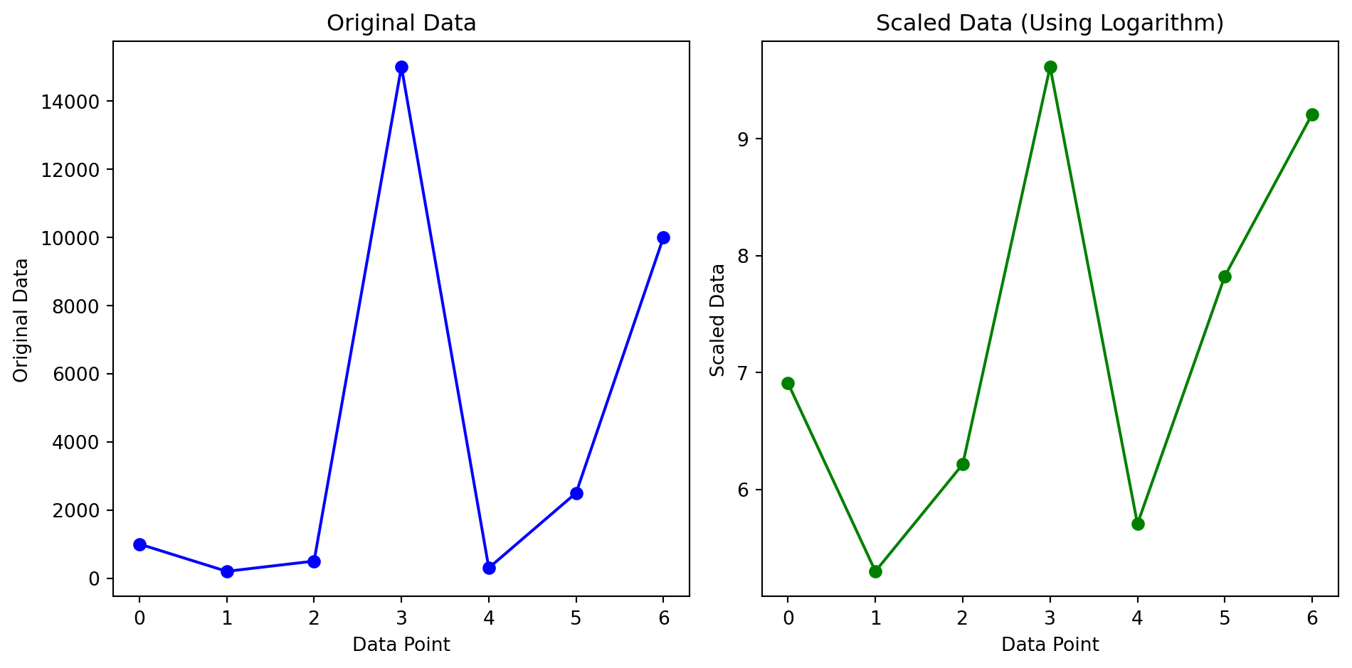
2. Data Scaling: In data analysis, data scaling is a preprocessing step used in data analysis to transform data to a similar scale. It helps avoid issues caused by having features with vastly different ranges. One common method of data scaling is using logarithms to scale down large numerical values.

Let’s demonstrate data scaling with a Python code example using the numpy library for numerical operations and the matplotlib library for visualization.

Code

import numpy as np
import matplotlib.pyplot as plt

# Sample data with a wide range of values
data = np.array([1000, 200, 500, 15000, 300, 2500, 10000])

# Apply data scaling using the natural logarithm (base e)
scaled_data = np.log(data)

# Plot original and scaled data
plt.figure(figsize=(10, 5))

# Plot original data
plt.subplot(1, 2, 1)
plt.plot(data, marker='o', linestyle='-', color='b')
plt.xlabel('Data Point')
plt.ylabel('Original Data')
plt.title('Original Data')

# Plot scaled data
plt.subplot(1, 2, 2)
plt.plot(scaled_data, marker='o', linestyle='-', color='g')
plt.xlabel('Data Point')
plt.ylabel('Scaled Data')
plt.title('Scaled Data (Using Logarithm)')

plt.tight_layout()
plt.show()

In this example, we have an array data containing some sample data with a wide range of values. To scale the data, we apply the natural logarithm (base \(e\)) to each element of the array using np.log(). The resulting scaled_data array contains the scaled-down values.

By using logarithms for data scaling, we transform the data into a more manageable range, making it easier to visualize and analyze. Data scaling is particularly useful in situations where the range of values is large and can help improve the performance of machine learning models and statistical analyses.

Relation with Summation

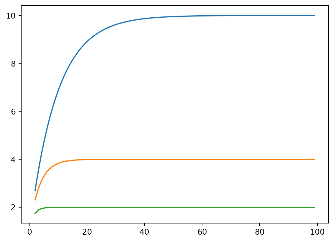
A geometric series is a specific type of summation in which each term is found by multiplying the previous term by a constant factor. The general form of a geometric series is:

\(\sum_{n=0}^{k} ar^n\)

Where \(a\) is the first term, \(r\) is the common ratio between consecutive terms, and \(n\) is the index variable. Geometric series are commonly used in various mathematical and financial applications.

Code

import matplotlib.pyplot as plt
import numpy as np

def geom_series(a, k):
  summation = sum(a**i for i in range(0, k+1))
  return summation

r1 = 0.9
r2 = 0.75
r3 = 0.5
x = np.arange(2, 100)
y1 = np.array([geom_series(r1, k) for k in x])
y2 = np.array([geom_series(r2, k) for k in x])
y3 = np.array([geom_series(r3, k) for k in x])
plt.clf()
plt.plot(x, y1)
plt.plot(x, y2)
plt.plot(x, y3)
plt.show()

Application in Valuation of Investments - Discounting Cash Flows:

In finance, summations and geometric series are utilized in discounted cash flow analysis to determine the present value of future cash flows, helping investors make informed decisions about their investments based on the time value of money. Discounted cash flow (DCF) analysis is a widely used method to determine the present value of future cash flows.

When a constant series of cash flows is expected to be received in the future (e.g., an investment that generates fixed returns over time), we can represent it as a geometric series. However, since money received in the future is not as valuable as money received today (due to the time value of money), we need to discount these future cash flows to their present value using an appropriate discount rate.

The present value (PV) of a series of future cash flows can be calculated using the geometric series formula:

\[ PV = C * (\frac{1}{(1 + r)^1} + \frac{1}{(1 + r)^2} + ... + \frac{1}{(1 + r)^k}) \]

\[ = C * \sum_{n=1}^{k} \frac{1}{(1 + r)^n} \] \[ = C*\frac{1-1/(1+r)^k}{r} \]

Where:

\(PV\) is the present value of the cash flows.
\(C\) is the constant cash flow received each period.
\(r\) is the discount rate (expressed as a decimal).
\(n\) is the number of periods (the investment horizon).

By discounting future cash flows back to their present value, we can compare investments with different time frames or cash flow patterns and make informed investment decisions.

Code

r = 0.1
a = 1/(1+r)
k = 5
a = geom_series(a, k) - 1
b = (1-(1/(1+r)**5))/r

print(a, b)

3.7907867694084487 3.7907867694084505

Assignment

Basic: Make a short video explaining how geometric series are used in financial valuation (discounted cash flow method). Do proper research and use code demos.

Stretch: Expand your video with an example of valuing the stock of a listed company. Compare your result with the actual market price and discuss the differences. Illustrate with code examples and charts. Provide a list of interesting resources on the matter.

Challenge: Share your content online (e.g. Linkedin or Medium), gather feedback and write a reflection on it.